Query Optimization Technology for Correlated Subqueries

This article mainly describes what correlated subqueries are and how to rewrite correlated subqueries as SQL queries in common semantics.
The background section explains the semantics of common correlated subqueries, the advantages of correlated subquery syntax, and the challenges to the database system during execution. The second section focuses on decorrelation, which refers to rewriting a correlated subquery as a common query. In Section Three, the optimization methods for decorrelation will be introduced.
Background
The correlated subquery is a subquery associated with the external query. To be specific, columns involved in the external query are used in the subquery.
Because of the flexibility of using correlated columns, it will greatly simplify SQL statement and make the SQL query semantics more understandable to rewrite an SQL query as a subquery. Several cases of using TPC-H schema below will make this point. The TPC-H schema is a typical database for the order system, containing tables such as the customer table, orders table, and lineitem table, as shown in the following figure.
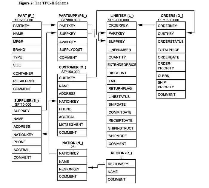
The correlated subquery can be used as a filter condition to query “the information of all customers who have never ordered”. The SQL statement written by using the correlated subquery is as follows. It can be seen that the “not exists” subquery uses the external column c_custkey.
-- Information of all customers who have never ordered
Select c_custkey
from
  customer
where
  not  exists (
    select
      *
    from
      orders
    where
      o_custkey = c_custkey
  )
If subquery is not used, the customer table and orders table need to be left joined first, and then the rows not joined need to be filtered out. The SQL query is as follows:
-- Information of all customers who have never ordered
select c_custkey
from
  customer
  left join (
    select
      distinct o_custkey
    from
      orders
  ) on o_custkey = c_custkey
where
  o_custkey is null
The example shows that the complexity of SQL statements is reduced and readability is improved by using correlated subqueries.
In addition to using correlated columns in “exists/in” subqueries, correlated subqueries can also be used in the where clause as values required for filtering conditions. For example, tpch q17 below uses subqueries to obtain an aggregation value as the filtering condition.
-- tpch q17
SELECT Sum(l1.extendedprice) / 7.0 AS avg_yearly
FROM   lineitem l1,
       part p
WHERE  p.partkey = l1.partkey
       AND p.brand = 'Brand#44'
       AND p.container = 'WRAP PKG'
       AND l1.quantity < (SELECT 0.2 * Avg(l2.quantity)
                         FROM   lineitem l2
                         WHERE  l2.partkey = p.partkey);
In addition, correlated subqueries can also be used anywhere the single line (scalar) is permitted, such as in the select list. The following SQL statements containing correlated subqueries can be used to summarize some customer information in a report and to query the total order amount for each customer.
-- Customer and corresponding total consumption
select
  c_custkey,
  (
    select sum(o_totalprice)
    from
      orders
    where o_custkey = c_custkey
    )
from
  customer
More complexly, for example, to query each customer and the corresponding total amount of orders they have been signed before a certain date, only a few changes are required by using correlated subqueries, shown as follows.
select
  c_custkey,
  (
    select
      sum(o_totalprice)
    from
      orders
    where
      o_custkey = c_custkey
      and '2020-05-27' > (
        select
          max(l_receiptdate)
        from
          lineitem
        where
          l_orderkey = o_orderkey
      )
    )
from
   customer
The convenience of using correlated subqueries is demonstrated in the examples above. However, the use of correlated subqueries poses many challenges on execution. To compute the correlated result value (the output of the subquery), the iterative execution method is required.
Take the abovementioned tpch 17 as an example.
SELECT Sum(l1.extendedprice) / 7.0 AS avg_yearly
FROM   lineitem l1,
       part p
WHERE  p.partkey = l1.partkey
       AND p.brand = 'Brand#44'
       AND p.container = 'WRAP PKG'
       AND l1.quantity < (SELECT 0.2 * Avg(l2.quantity)
                         FROM   lineitem l2
                         WHERE  l2.partkey = p.partkey);
The subquery here uses the column p.partkey of the external query.
SELECT 0.2 * Avg(l2.quantity)
FROM   lineitem l2
WHERE  l2.partkey = p.partkey  -- p.partkey is a column of external query
The optimizer displays the query logic as the following logic tree.
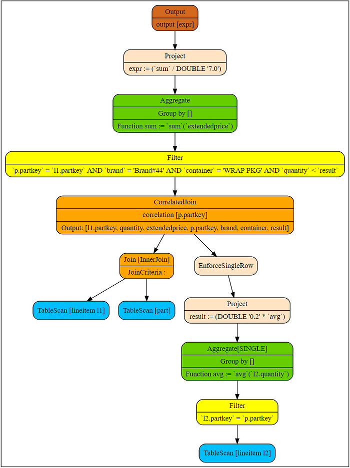
If the database system cannot view logic tree, the physical plan can be viewed via explain command. Generally, the output is as follows.
+---------------+
| Plan Details  |
+---------------+
 1- Output[avg_yearly] avg_yearly := expr
 2    -> Project[] expr := (`sum` / DOUBLE '7.0')
 3        - Aggregate sum := `sum`(`extendedprice`)
 4            -> Filter[p.`partkey` = l1.`partkey` AND `brand` = 'Brand#51' AND `container` = 'WRAP PACK' AND `quantity` < `result`]
 5                - CorrelatedJoin[[p.`partkey`]]
 6                    - CrossJoin
 7                        - TableScan[tpch:lineitem l1]
 8                        - TableScan[tpch:part p]
 9                    - Scalar
10                        -> Project[] result := (DOUBLE '0.2' * `avg`)
11                            - Aggregate avg := `avg`(`quantity`)
12                                -> Filter[(p.`partkey` = l2`partkey`)]
13                                    - TableScan[tpch:lineitem l2]
The operator connecting external queries and subqueries is called CorrelatedJoin, which is also known as lateral join and dependent join. The left subtree is called external query (input), while the right subtree is called subquery. External columns that appear in the subquery are called correlated columns. The correlated column in the example is p.partkey.
The following figure shows the corresponding logic plan and related definition in this example. In the results returned by the explain command, the sixth to eighth rows are external queries while the ninth to thirteenth are subqueries. The correlated part is in the filter in the twelfth row.
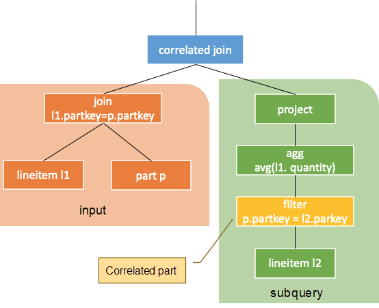
The output of this operator is equivalent to the result of iterative execution. In other word, the values of each correlated column in the left subtree are computed in the right subtree with a row of results returned. The subquery can serve as a user-defined function (UDF), while the value of the correlated column of the external query as the input parameter for this UDF. Note that the subquery needs to be certain. That is, for the correlated columns with the same value, the results returned by subqueries should be certain as well.
In the above example, if the external query has a row of p.partkey whose value is 25, the corresponding output of the correlated join operation for this row is as follows.
-- When p.partkey = 25, the corresponding subquery is
SELECT 0.2 * Avg(l2.quantity)
FROM   lineitem l2
WHERE  l2.partkey = 25
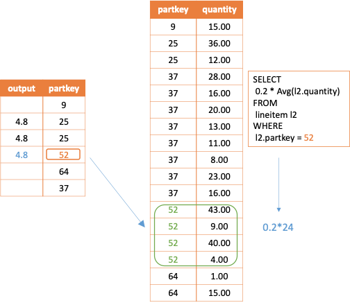
Note that if no result is queried, a null row is returned. If more than one row of results is returned by subqueries in running, a runtime error should be reported. In the logic plan, the node enforcesinglerow is used for execution control.
It can be seen from the above description that the operator CorrelatedJoin eliminates the previous top-down execution mode of the logic tree. A common logic tree is executed from the leaf node to the root node. However, the row values in the left subtree of CorrelatedJoin will be brought to its right subtree and executed repeatedly.
The correlatedjoin node adds a column to the result of the external query.
This iterative execution method is as complex as performing cross join operation on the tree before the external query and the subquery are associated.
In addition, such iterative execution is a great challenge to a distributed database system since the scheduling logic in execution needs to be modified. If the results are not cached for this execution method, calculations with repeated results will be performed.
The traditional optimizers do not optimize Correlatedjoin node in particular. In order to support the iterative execution of correlated subqueries, optimizers perform equivalence conversion on the Correlatedjoin operator in the initial phase. The transformed logic tree computes the correlated subquery results by using common operators such as join and aggregation. This process is called decorrelation or unnesting. The following section mainly describes common decorrelation methods.
Common Decorrelation Methods
For convenience, this section will only discuss scalar correlated subqueries, which output a column of values.
Before discussing about decorrelation, the characteristics of correlation subquery output are summarized as follows.
- The correlated join operator adds a column to the external query result.
- The result of the added column is obtained by computing the value of the correlated column of the external query in the subquery. If more than one row of computing results is added, an error is reported. Null computing result should also be added.
- Unlike the join operator, the correlated join operator does not change other columns of the external query, that is, the row quantity is not changed.
The key to decorrelation is to obtain the values of the corresponding columns of the external query for subqueries.
It is manifested in the plan to push the correlated join operator down below the correlation part on the right. When the left and right subtrees of a correlated join operator do not have correlated columns, the correlated join operator can be converted into a join operator. In this way, the subquery can obtain the values of the correlated columns by joining with the external query. Thus, the computation can be performed from top to bottom as original. As shown in the following figure, the rest subquery runs before the correlation part. When the correlated join operator is pushed down to the correlation part, it can be converted into a common join operator.

After the correlated join operator is pushed down, the operators above the correlation join need to be rewritten to maintain equivalence. As shown in the figure above, subquery is changed to subquery’.
Pushdown Rules
The equivalence conversion rules of pushing the correlatedjoin* operator down to other operators (such as filter, project, aggregation, and union) are given in the paper Orthogonal Optimization of Subqueries and Aggregation5.
However, the correlatedjoin* operator filters the number of rows of the external query, which is similar to inner join (called

in the paper). In this article, a more general correlatedjoin operator (called

in the paper), which is similar to left join, is discussed. This article also discusses what needs to be rewritten to ensure that the number of rows in the external query are not filtered.
Due to space limitation, the following part describes only the equivalence conversion rules for pushing the correlated join operator down to filter, project, and aggregation operators.
For simplicity, enforcesinglerow is removed from the logic tree.
Conversion Rule One: Conversion to Join Without Correlation
As mentioned earlier, the left subtree of correlated join operator is input and the right subtree is subquery. When the left and right subtrees of the correlated join are not correlated, the subquery results are the same for each row of the external query.
The correlated join operator can be converted into common left join operator without join criteria.

Note: enforcesinglerow must be added to the subquery to ensure that the semantics of the join operator are the same as that of correlated join. That is, the input will not inflate.
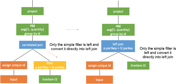
Conversion Rule Two: Conversion to Join with Simple Correlation Conditions
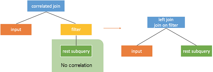
When the top node in the right subtree of the correlated join is a correlated filter without correlation beneath, the filter can directly serve as a criteria of the left join. It can also be understood as filter lifting, as shown in the following figure.
Conversion Rule Three: Pushdown through Filter
According to the paper, correlatedjoin* can be directly pushed down through the filter. However, if correlatedjoin is to be pushed down, the filter needs to be rewritten as a project with "case when". If the rows in the subquery do not meet the filter conditions, the output value is null.

Conversion Rule Four: Pushdown through Project

An output column of the input needs to be added in project to push correlated join through the project.
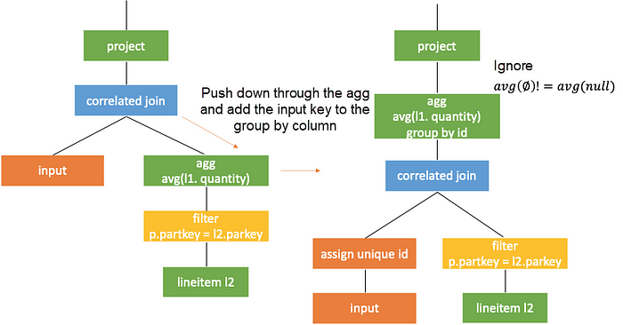
Conversion Rule Five: Pushdown through Aggregation
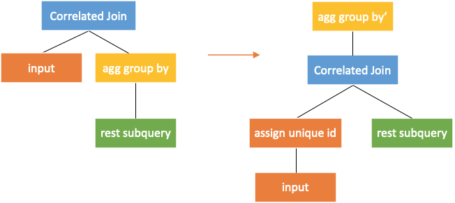
The aggregation group by operator needs to be rewritten when the correlated join is pushed down through.
All columns of the external query should be added to the columns output by the aggregation group by operator. Key is required for the external query. If no key exists, a temporary key needs to be generated. The operator that can generate keys is assignuniqueid in the following figure.
For global aggregation, additional processing is required, as shown in the following figure.
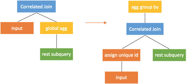
When pushing correlated join down to the global aggregation, an input column with key is added as the column for the aggregation group by. The prerequisite for this rule is that the aggregation function must satisfy

. That is, the calculation results of the empty set and the null set by aggregation function must be the same.
Note: In MySQL and AnalyticDB for MySQL (ADB) syntax, count does not meet this requirement. ADB is a cloud native data warehouse exclusively developed by Alibaba Cloud and is compatible with MySQL syntax. The count value of an empty set is 0, while the count value of any set containing null values is not 0. Therefore, each row in the subquery should be marked and the empty set should be specially dealt with. Details are not provided here.
The paper Orthogonal Optimization of Subqueries and Aggregation[1] repeatedly pushes correlated join down based on these rules until it is converted into common join.
Take the previous tpch q17 as the example again. Push correlated join down to project in the subquery first, and the query is as follows.
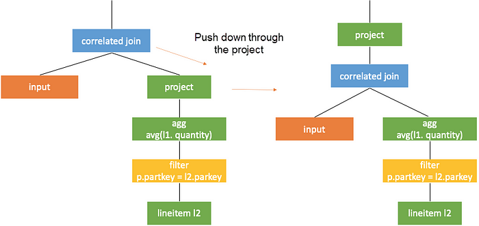
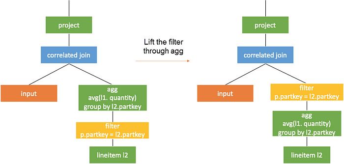
Then, push correlation join through agg and rewrite agg, as shown in the following figure. Here,

is ignored. Otherwise, all rows in the subquery need to be marked. The empty set is to be processed specially after the correlated join operation based on the subquery results and marked values. The values of marked rows turn from null to 0.
Those who are interested can view the final plan of tcph q17 in the next section.
Then, lift the filter directly according to the second rule mentioned previously. As such, the query becomes a common one without correlation.
Reuse the Results
It is known from the previous section that the result of a subquery is computed with the value of the correlated column assigned to each row. Then, the results of correlated columns with same values are completely the same after calculated in the subquery. In the example above, the subquery output of correlatedjoin for the same p.partkey values is the same. As shown in the following figure, if the value of the external query partkey is 25, the generated correlated subqueries are the same and so are the results.
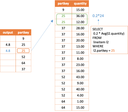
Newmann’s paper Unnesting Arbitrary Queries [1] in 2015 has introduced a method. First, obtains the distinct from the correlated column in the external query. Then, performs left join operation on the value returned by correlated join and the external query based on correlated columns, as shown in the following figure.
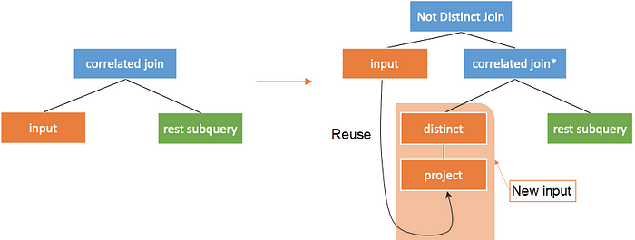
The condition of not distinct join here corresponds to <=> in MySQL. The result of null <=> null is true, so the returned value and the external query can be joined together.
For the preceding example, as shown in the following figure, perform distinct operation on the correlated column partkey of external query first. Then, assign the value of the correlated column to the subquery and compute. Finally, join the corresponding results to the original external query.
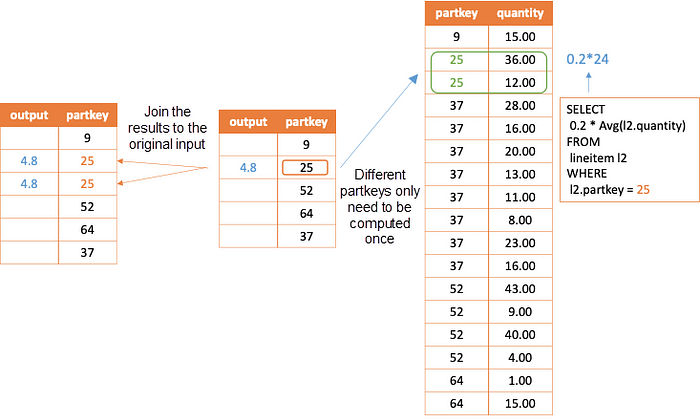
If the above conversion is performed, it can be considered that the correlated column of the new input is always distinct. Now, the correlatedjoin* operator allows input columns to be filtered. In addition to avoiding repeated subqueries on the same column, this method has the following advantages:
- New external queries always have keys since the distinct operation has been performed.
- The
correlatedjoin*operator filters the external query columns, so its pushdown is simpler, which does not require the assign unique id or retain all rows.
After the above conversion, correlatedjoin* can be pushed down to a place where no correlation in the left and right subtrees exists. Thus, it can be converted into an inner join based on equivalence pushdown rules.
If decorrelation is performed according to the method in Unnesting Arbitrary Queries[1], some result of the input need to be reused, which requires support from the execution engine. It should be noted that when the system does not support reuse, the input subtree needs to be executed twice, as shown in the following figure. In this case, the results of the input subtree need to be deterministic. Otherwise, this method cannot be used for decorrelation.
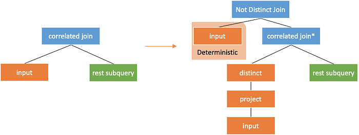
Optimization of Correlated Subqueries
The optimizer of ADB matches and converts the logic plan based on each conversion rule. This means that after the decorrelation, it is unnecessary to worry about the efficiency of the plan generated. The plan can be directly optimized. However, the reality is that the subsequent rules are not perfect, and the relationship between the external query and the subquery is broken after the decorrelation. It is hoped that the plan is optimized as much as possible during decorrelation.
Correlated Subqueries of exists/in/filter
For simplicity, only the scalar subqueries are discussed about in the previous section. The exists and in subqueries can also be rewritten as scalar subqueries. For example, exists subqueries can be rewritten as count(*) > 0.
However, if the results returned by the subquery are used to filter rows of the external query, the entire decorrelation process will actually be simplified. Therefore, subqueries such as exists and in are specially processed and distinguished in syntax parsing. During the decorrelation process, decorrelate them directly by using semijoin/antijoin operators if possible. Otherwise, they will convert into scalar subqueries with correlated join.
Lifting of Correlated Conditions
It can be seen that the logic tree becomes more complicated with the pushdown of correlated join. So, the correlated operators in the subquery are lifted before pushdown of correlatedjoin. In this case, the higher the correlated operator is, the faster the correlatedjoin is pushed down below the correlated part. Take the following query as an example:
SELECT t1.c2
FROM
  t1
WHERE t1.c2 < (
    SELECT 0.2 * max(t2.x)
    FROM
      t2
    WHERE t2.c1 = t2.c1
    GROUP BY t2.c1
  );
Since t2.c1 = t2.c1 can be lifted up above agg, which is a condition on the agg group by column for subquery, the following conversion can be implemented. First, lift the correlated filter (sometimes it needs to be rewritten). Then, push the correlatedjoin through filter and apply the conversion rule two.

A more specific example is the tpch q17 mentioned earlier. The scalar subquery as the filter condition can also be further rewritten.
The following figure shows the logic plan after pushing down the correlated join and rewriting it as left join based on the conversion rules.
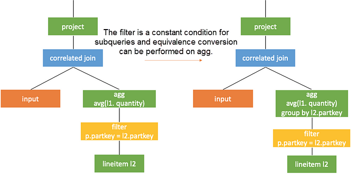
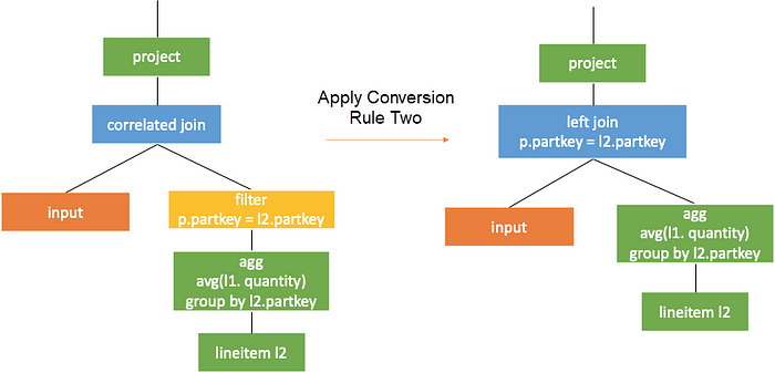
The scalar subquery serves as a filter condition. As such, the subquery does not return null result and the corresponding external query will definitely be filtered out. So, correlatedjoin can be directly converted into correlatedjoin*. Along with the filter lifting, the following plan can be obtained. The advantage is that aggregation (early agg) can be performed before join. As to the disadvantage, semantic inequivalence and count bug are easily to occur.
Cost-related Subquery Optimization
Decorrelation with Window Operator
It is impressive that the correlatedjoin operator adds a column to the external query, which is similar to the window operator. The semantics of window operator is to add a value computed in the window frame to each row, without changing the number of input rows. Therefore, the window operator can be used for decorrelation. If interested, see Enhanced Subquery Optimizations in Oracle[4] and WinMagic: Subquery Elimination Using Window Aggregation[3].
For rewriting after decorrelation, window operators are directly used to connect the subquery results to the external query, when the external query contains all the tables and conditions in the subquery. It is helpful for saving a lot of tablescan operations. Take the rewriting of tpch q2 as an example, as shown in the following figure.
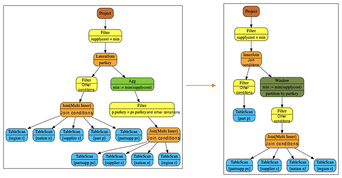
Agg can be rewritten as window because the external query includes all tables and conditions of the subquery. Additionally, the agg function min satisfies

. If not, the rows need to be marked and the output needs to be rewritten by using case when statement.
The number of tablescan operations after the rewriting is notably reduced. Moreover, the subsequent optimization rules exchanges the order of join and window according to the information of primary key and the characteristics of agg function. This further reduces the amount of data (filter-join pushdown) input by window operators.
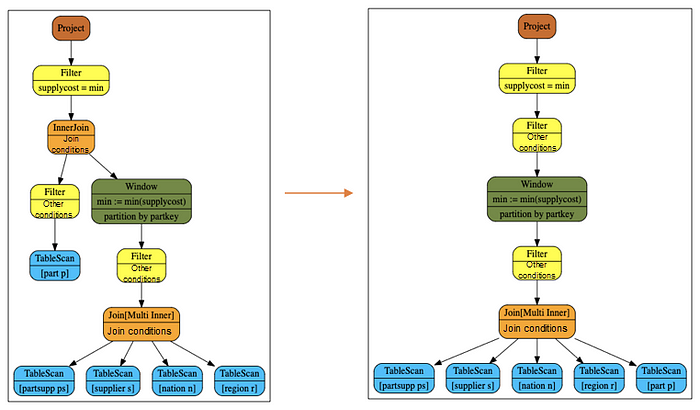
The benefits have been discussed about in many articles. This article describes the defects of such rewriting.
- If the private key does not indicate that the agg function is sensitive to duplicates, the window operator will block the filter-join pushdown. This interrupts joingraph, thus increasing the intermediate result of join.
- For rewriting as a join with two subtrees, the filter-join can be pushed down to one of the subtrees. However, the filter-join cannot be pushed down after rewriting as window.
- If the pipeline execution model or cte is used, table scanning produces limited benefits.
- The optimization processing of traditional optimizers for join and agg are much better than for window and the optimization rules are much richer.
To sum up, it is necessary to estimate the benefit and cost when using window to rewrite a correlated subquery.
Correlated Join Pushdown in External Queries
Before pushing down correlatedJoin towards the subquery, correlatedjoin is pushed down first in the external query. For example, it is pushed down through cross join etc.
The correlatedJoin operator will never cause data expansion, so, theoretically, the pushdown should be done earlier. In fact, correlatejoin pushdown may also split the joingraph, thus bringing about the similar problems of window rewriting.
Use of Equivalent Columns
If the subquery has a column equivalent to columns in the external query, this column can be used to rewrite the correlated column in subquery. This can reduce the quantity of correlated parts and simplify the query. The following part is a simple example.
Select t1.c2
From
  t1
Where
  t1.c3 < (
    Select min(t2.c3)
    From t2
    Where t1.c1 = t2.c1
    group by t1.c1
  )-- Replace t1.ct with t2.c1 in subquery for simplificationSelect t1.c2
From
  t1
Where
  t1.c3 < (
    Select min(t2.c3)
    From t2
    Where t1.c1 = t2.c1
    group by t2.c1
  )
Subquery Related Optimization Rules
On the one hand, the characteristics of the correlatedjoin operator provide some information for optimization. For example:
- The row number after the
correlatedjoinoperator is the same as that in the left subtree. - The output of enforcesinglerow is one row.
- The correlated column of the external query determines the newly added output column of
correlatedjoin. This is called function dependency. - The key generated by the assign unique id has unique attributes and can be used for subsequent simplification of aggregation and group by.
- The meaningless sort operations in the subquery can be filtered.
On the other hand, during subquery rewriting, subqueries can be simplified through attribute deduction. For example:
- There is no need to add the uniqueid column to the originally unique external query.
- Tailoring is allowed when the output of enforcesinglerow sub-node is always one row.
- Some subqueries with the correlated column on the project can be rewritten as exists subqueries in some cases.
sql select t1.orderkey, ( select min(t1.orderkey) from orders t2 where t2.orderkey > t1.orderkey ) from orders t1 order by 1Notes:
Pay attention to the following two aspects when decorrelating subqueries: adding one column only to the external query and dealing with null values.
Count bug
This is a typical mistake in decorrelation mentioned frequently in literature. For example, in the following query, the prerequisite is that t1.c3 is less than 0. In this case, the correlation conditions where the subquery is involved in should have no filter degree, while some rows are filtered after rewriting as inner join. It is not semantically equivalent.
Select t1.c2
From
  t1
Where
  t1.c3 < (
    Select COUNT (*)
    From t2
    Where t1.c1 = t2.c1
  )
Distributed LeftMarkJoin
LeftMarkJoin[2] in the paper Unnesting Arbitrary Queries[1] is also error-prone. Its output is the same as the semantics of the in clause. That is, its output is as follows.
select t1.c1
    in (
    select
      t2.c1
    from
      t2)
from
  t1
The logic plan for this query is as follows:
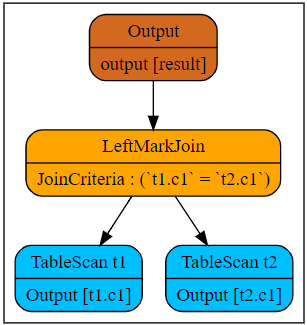
It adds a column of in clause to the result of the left subtree, which may be true, false, or null.
In a distributed environment, repartitioning and writing this operator to disk will easily cause errors in the calculations related to null values.
For example, if LeftMarkJoin is the execution method of repartitioning, it reshuffles the data in the left and right tables according to the hash value of c1. As such, the null rows in t1.c1 will be shuffled to the same executor. If no data in the right table is shuffled to this executor, the executor cannot decide whether to output null or false for these null rows. It is because the result of null in empty set is false, while the results of other null in sets are null. In this case, the executor does not know whether the right table is empty.
Efficiency after decorrelation
The iterative execution is mentioned at the beginning. Here are more explanations. Even if the correlation is decorrelated into operators such as join or agg, for some correlated subqueries, cross join is also required to compute the query results.
There are two examples. The first one is a common correlated subquery which can be converted into inner join and early agg. As to the second query, it becomes an inequivalent condition of left join on after decorrelation, which is the same as cross join in cost.
-- sql 1
SELECT t1.c1
  FROM t1
 WHERE t1.c2 > (
   SELECT min(t2.c2)
     FROM t2
    WHERE t2.c1 = t1.c1
   );-- sql 2
SELECT t1.c1
  FROM t1
 WHERE t1.c2 > (
   SELECT min(t2.c2)
     FROM t2
    WHERE t2.c1 > t1.c1
   );
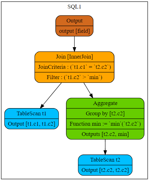
The following figure shows the plan after SQL1 is decorrelated.
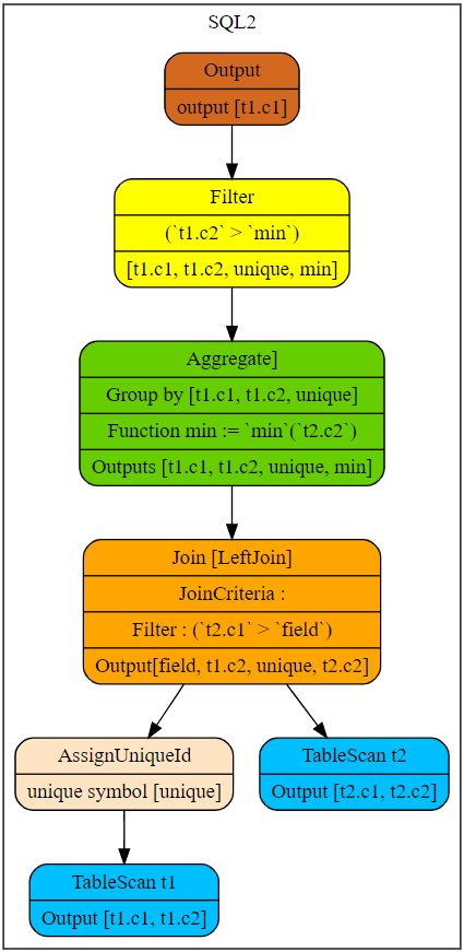
The following figure shows the plan after SQL2 is decorrelated.
For SQL1, semantically, the cost is the same as that of inner join on equivalent condition, since the scanned rows in the subquery and each row of the external query assigned to the subquery do not overlap. Besides, the results of min function in the subquery for the same external rows are the same. So, early agg can be applied for further optimization.
For SQL2, semantically, all rows in the external query need to be assigned to the subquery and then scanned with each row of the subquery. By doing so, the output can be determined when the subquery satisfies t2.c1 > t1.c1. The cost of computing cannot be reduced through optimization. Fortunately, the output is always the same for the same t1.c1. So, the reuse of results mentioned in Unnesting Arbitrary Queries[1] can still provide optimization.
References
- Neumann, Thomas, and Alfons Kemper. “Unnesting arbitrary queries.” Datenbanksysteme für Business, Technologie und Web (BTW 2015) (2015).
- Neumann, Thomas, Viktor Leis, and Alfons Kemper. “The Complete Story of Joins (inHyPer).” Datenbanksysteme für Business, Technologie und Web (BTW 2017) (2017).
- Zuzarte, Calisto, et al. “Winmagic: Subquery elimination using window aggregation.” Proceedings of the 2003 ACM SIGMOD international conference on Management of data. 2003.
- Bellamkonda, Srikanth, et al. “Enhanced subquery optimizations in oracle.” Proceedings of the VLDB Endowment 2.2 (2009): 1366–1377
- Galindo-Legaria, César, and Milind Joshi. “Orthogonal optimization of subqueries and aggregation.” ACM SIGMOD Record 30.2 (2001): 571–581.
- Galindo-Legaria, C. A. “Parameterized queries and nesting equivalences.” Technical report, Microsoft, 2001. MSR-TR-2000–31, 2000.


